2. Data in R

Motivating scenario: You understand the very basics of R, and can load data into it. But now you want to actually do things!
Learning goals: By the end of this chapter you should be able to
- Explain the tidy data format and differentiate between tidy and untidy data.
- Use the
select()function inRto choose columns to work with.
- Use the
mutate()function inRto add or over-write columns.
- Use the
summarize()function inRto summarize the data.- And doing so by groups with the
group_by()function.
- And doing so by groups with the
- Use the
filter()function to choose the rows you want to work with.
- Combine these operations with the pipe
|>operator.
Tidy data
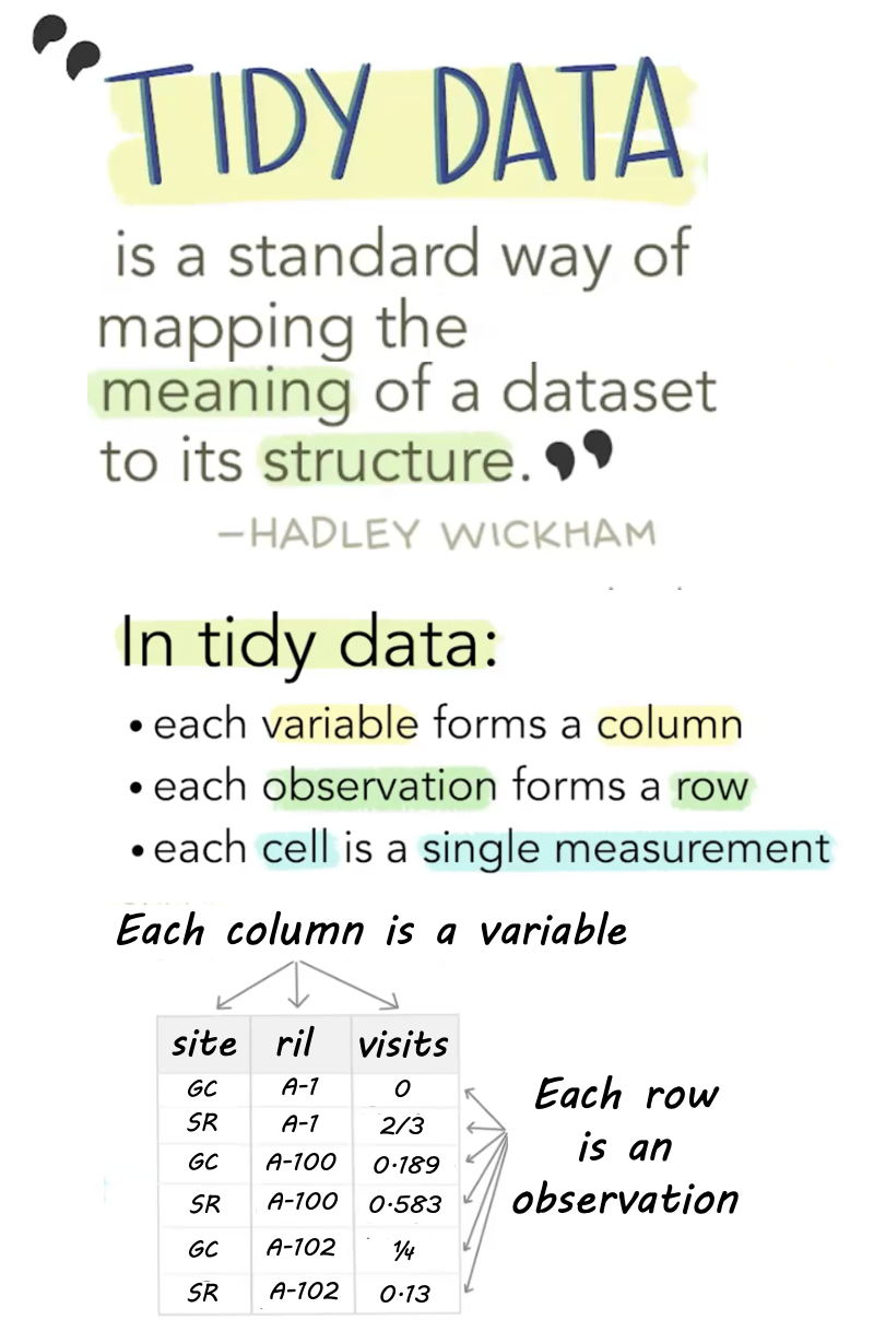
Like families, tidy datasets are all alike but every messy dataset is messy in its own way. Tidy datasets provide a standardized way to link the structure of a dataset (its physical layout) with its semantics (its meaning).
Hadley Wickham. Tidy data. Wickham (2014).
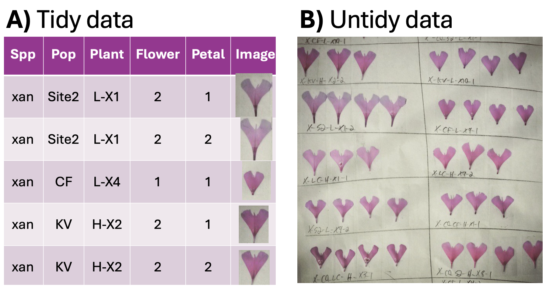
Data can be structured in different ways: in a tidy format, each variable has its own column, and each row represents an observation. In contrast, messy data might combine multiple variables into a single column or store observations in a less structured format. Figure 2 A shows “long” data with one variable per column. Figure 2 B contains boxes (rather than rows or columns) with petals from a given flower laid out neatly, and information about the flower and plant written beneath it. Both formats have their costs and benefits:
- Figure 2 A is “tidy”: Each row is an observation (a petal), and each column is a variable related to that observation. Because this style is so predictable, this format simplifies computational analyses.
- Figure 2 B is not “tidy”: There are not simple rows and columns, and variables are combined in a long string. This format is useful in many ways—for example, humans can easily identify patterns, and data can be stored compactly.
Note that the tidy data format is not necessarily “prettier” or easier to read – in fact, in visual presentation of data for people, we often choose an untidy format. But when analyzing data on our computer, a tidy format simplifies our work. For this reason we will work with tidy data when possible in this book.
Because all untidy data are different, there is no way to uniformly tidy an untidy dataset. However, the tidyr package has many useful functions. Specifically, the pivot_longer() function allows for converting data from wide format to long format.
Tibbles
A tibble is the name for the primary structure that holds data in the tidyverse. A tibble—much like a spreadsheet—does not automatically make data tidy, but encourages a structured, consistent format that works well with tidyverse functions.
In a tibble, each column is a vector. This means that all entries in a column must be of the same class. If you mix numeric and character values in a column, every entry becomes a character.
In a tibble, each row unites observations. A row can have any mix of data types.
Tibbles vs. Data Frames For base R users – A tibble is much like a data frame, but some minor features distinguish them. See Chapter 10 of Grolemund & Wickham (2018) for more info.
| Feature | Tibble | Data Frame |
|---|---|---|
| What you see on screen | First ten rows & cols that fit | Entire dataset |
| Data Types Displayed | Yes – <dbl>, <chr>, etc | No |
| Subsetting to one column returns | A tibble | A vector |
The read_csv() function that we introduced earlier to load data imports data as a tibble. Looking at the data below, you are probably surprised to see that growth rate is a character <chr>, because it should be a number <dbl>. A little digging reveals that the entry in the third row has a growth rate of 1.8O (with the letter, O, at the end) which should be 1.80 (with the number 0 at the end)
library(readr)
library(dplyr)
ril_link <- "https://raw.githubusercontent.com/ybrandvain/datasets/refs/heads/master/clarkia_rils.csv"
ril_data <- readr::read_csv(ril_link)
ril_data
# A tibble: 593 × 17
ril location prop_hybrid mean_visits growth_rate petal_color petal_area_mm
<chr> <chr> <dbl> <dbl> <chr> <chr> <dbl>
1 A1 GC 0 0 1.272 white 44.0
2 A100 GC 0.125 0.188 1.448 pink 55.8
3 A102 GC 0.25 0.25 1.8O pink 51.7
4 A104 GC 0 0 0.816 white 57.3
5 A106 GC 0 0 0.728 white 68.6
6 A107 GC 0.125 0 1.764 pink 66.3
7 A108 GC NA NA 1.584 <NA> 51.5
8 A109 GC 0 0 1.476 white 48.1
9 A111 GC 0 NA 1.144 white 51.6
10 A112 GC 0.25 0 1 white 89.8
# ℹ 583 more rows
# ℹ 10 more variables: date_first_flw <dbl>, node_first_flw <dbl>,
# petal_perim_mm <dbl>, asd_mm <dbl>, protandry <dbl>, stem_dia_mm <dbl>,
# lwc <dbl>, crossDir <chr>, num_hybrid <dbl>, offspring_genotyped <dbl>Let’s get ready to deal with data in R
The following sections introduce the very basics of R including:
Then we summarize the chapter, present practice questions, a glossary, a review of R functions and R packages introduced, and present additional resources.