Motivating Scenario: You have a dataset with many variables (e.g. Numerous phenotypes, climatic variables, RNA-Seq, large scale genomic or phenomic data, OTU counts etc…) and want to broadly summarize variability in this dataset and the associations between these many variables. However, there are too many variables to interpret with simple plots or pairwise comparisons. You need a way to summarize the patterns of variation across all traits simultaneously.
Learning Goals: By the end of this chapter, you should be able to:
Understand what ordination methods like PCA and NMDS do
Explain the goals of PCA and NMDS in summarizing multivariate patterns.
Interpret PCA results in biological terms
Describe how traits combine to form principal components
Quantify how much variance is explained by each component
Understand and compare PCA and NMDS
Know when PCA is appropriate and when NMDS might be better
Anticipate and avoid common pitfalls
Handle missing data, decide whether to scale variables, and recognize when you’re double-counting information
Nowadays biologists are drowning in data. A single study, can include measurements of dozens of traits. Grinding up samples and running them through various machines provides us with genotypes at millions of loci, measures of gene expression across tissues, characterization of the thousands of microbes in a sample etc. Trying to interpret each variable on its own quickly becomes overwhelming — and looking at pairs of traits one at a time misses the bigger picture. So, we use multidimensional techniques to summarize how individuals differ across all traits simultaneously.
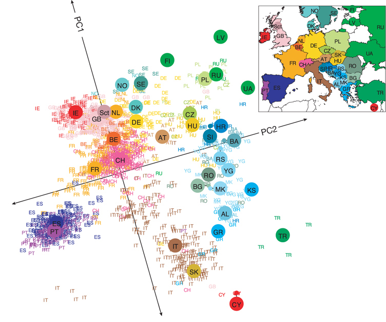
Principal Components Analysis (PCA) of genetic variation in Europe. This plot shows individuals sampled from across Europe, positioned along the first two principal components derived from genome-wide genetic data. Each point represents an individual, color-coded by country, with country codes overlaid. Strikingly, the resulting PCA plot recapitulates the geography of Europe, with spatial proximity on the map corresponding to genetic similarity. The inset shows actual country locations for reference. The work is from Novembre et al. (2008), and the image is from John’s website.
A common set of tools, known as ordination methods, summarize high-dimensional datasets into a few major axes of variation. These summaries can be incredibly informative, revealing key patterns in the data. For example, John Novembre showed that summarizing whole-genome data by its major axes of variation revealed a structure in European genetic variation that closely mirrors the geographic map of Europe. This example highlights the best of ordination methods because it:
Reduced high-dimensional data to a few informative axes.
Visualized relationships among individuals or species in a lower-dimensional space.
Highlighted the biological structure in multivariate datasets.
Let’s get started with ordination!
We will work through the intuition and mechanics of how to conduct a few standard ordination techniques. Our focus will be on building a conceptual understanding and a pragmatic “know-how”, rather than a rigorous mathematical foundation. Along the way, we’ll also wrestle with practical questions. For example “What do we do about missing data?”, “Should we scale our variables?”, and “When are two variables redundant? (and why should I care?)”
We’ll begin with Principal Component Analysis (PCA) — a linear method that looks for the directions of greatest variance in your data. We will start with a familiar dataset: Clarkia individuals from the GC site, for which we’ve measured anther-stigma distance, petal area, and leaf water content. These traits may relate to different aspects of plant performance or pollination biology — but PCA won’t “know” that. It will simply tell us how plants vary. We will then expand to other data sets to show what we can learn from a PCA.
Next we’ll explore Principal Coordinates Analysis (PCoA), which begins with a distance matrix rather than raw trait values. This makes it more flexible than PCA: you can use PCoA with ecologically-informed distance measures. While PCA is essentially an eigen-decomposition of the variance–covariance (or correlation) matrix, PCoA performs a similar decomposition of an arbitrary distance matrix, allowing us to apply ordination to data that might not meet PCA’s assumptions.
Finally, we’ll turn to Non-metric Multidimensional Scaling (NMDS), which takes does not assume linear relationships or focus on preserving absolute distances. Instead, it tries to preserve the rank order of distances between individuals — making it especially useful for messy ecological data, abundance counts, and presence-absence matrices. While NMDS is less mathematically pretty, it can be applied to ugly, real world biological data.
Novembre, J., Johnson, T., Bryc, K., Kutalik, Z., Boyko, A. R., Auton, A., Indap, A., King, K. S., Bergmann, S., Nelson, M. R., Stephens, M., & Bustamante, C. D. (2008). Genes mirror geography within europe. Nature, 456(7218), 98–101. https://doi.org/10.1038/nature07331