Motivating Scenario: You’ve used PCA to summarize variation in multivariate trait data, created biplots, and interpreted the results. But now you’re wondering: What is PCA actually doing behind the scenes? Where do principal components come from? What roles do centering and scaling play? etc…
Learning Goals: By the end of this subchapter, you should be able to:
Understand how PCA works.
Know that PCA is based on the eigen decomposition of a covariance (or correlation) matrix.
Recognize that PCs are linear combinations of original variables, oriented to capture the most variance.
Construct and interpret a covariance. Calculate covariance and correlation matrices in R.
See how PCA results connect to major patterns of variation through the covariance matrix. Explore how the main outputs of PCA—directions of variation and how much variation they explain—can also be generated using the eigen() function in R.
Compare scaled and unscaled PCA.
Understand how scaling affects the covariance structure and PCA results.
Interpret differences in PC loadings and variance explained with and without scaling.
How PCA Works
We just ran a PCA, looked at plots, and interpreted what the axes meant in terms of traits in our parviflora RILs. We also introduced the core idea: PCA finds new axes — principal components — that are combinations of traits, oriented to explain as much variation as possible. These components are uncorrelated with one another, and together they form a rotated coordinate system that helps us summarize multivariate variation.
The description of PCA and interpretation of results presented in the previous chapter are the bare minimum we need to understand a PCA analysis. Here, we will go beyond this bare minimum – dipping into the inner workings of PCA to better understand how it works and what to watch out for. This is essential for critically interpreting PCA results. A challenge here is that there is a bunch of linear algebra under the hood – and while I love linear algebra, I don’t expect many of you to know it. So, we will try to understand PCA without knowing linear algebra.
We will look at the two key steps in running a PCA.
Making a covariance (or correlation) matrix.
Finding Principal Components.
Code for selecting data for PCA from RILs planted at GC
After removing categorical variables from our data, the first step in PCA (if we do this without using prcomp()) is to build a matrix that shows the association between each trait in our data set.
We usually want to give each trait the same weight so we either center and scale (for each value of a trait we subtract the mean and divide by the trait’s standard deviation) and then find the covariance between each trait with the cov() function.
Making a covariance matrix from a centered and scaled data set, provides the exact same result as making a correlation matrix from the original data with the cor() function. So sometimes people talk about PCs from the correlation matrix (i.e. centered and scaled data), or the covariance matrix (i.e. centered but not scaled data).
# Scaling the datascaled_gc_rils_4pca <- gc_rils_4pca |>select(-made_hybrid)|># Remove categorical variablesmutate_all(scale) # Subtract mean and divide by SD# Finding all pairwise covariances on centered and scaled datacor_matrix <-cov(scaled_gc_rils_4pca)
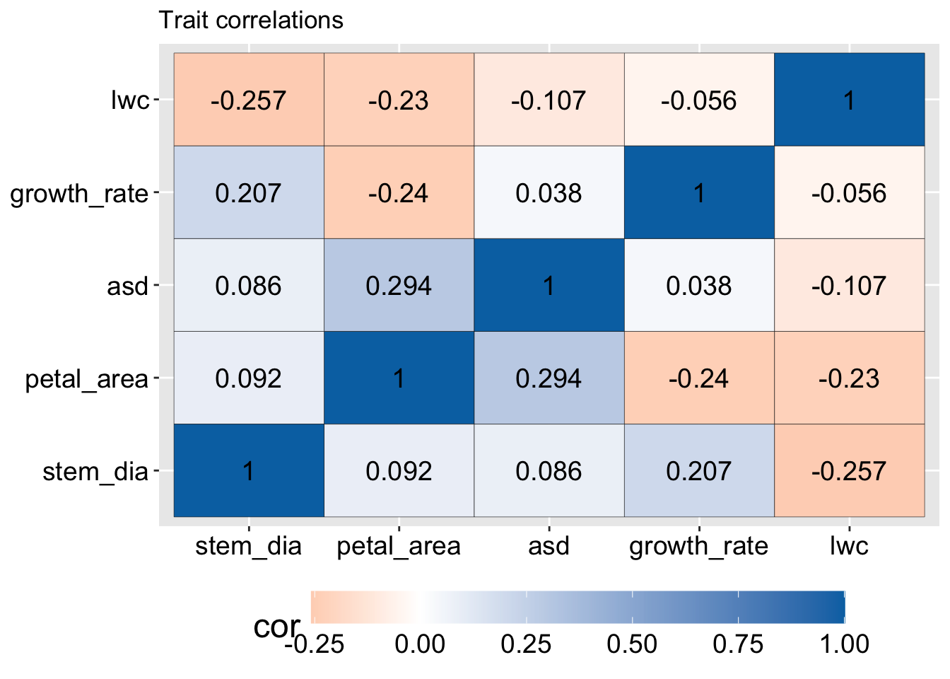
A few simple patterns jump out from this correlation matrix:
All values on the diagonal equal one. That’s because all traits are perfectly correlated with themselves (this is true of all correlation matrices).
The matrix is symmetric – values on the bottom triangle are equal to those on the top triangle (this is also true of all correlation matrices).
Some traits are positively correlated with each other – e.g. there is a large correlation between anther stigma distance and petal area – perhaps because they both describe flower size.
Some traits are negatively correlated with each other– e.g. nearly all other traits are negatively correlated with leaf water content.
Figure 1: Pairwise correlations among traits in parviflora recombinant inbred lines. Each cell shows the covariance of scaled and centered data (i.e. correlation) between two traits, with color indicating strength and direction of association (blue = positive, orange = negative). Traits include stem diameter, petal area, anther–stigma distance (asd), growth rate, and leaf water content (lwc). The matrix is symmetric, and all diagonal values are 1 by definition.
Finding Principal Components
In PCA, we’re trying to find new axes that summarize the patterns of variation in our dataset. These principal components are chosen to explain as much variance as possible. As we have seen, each principal component is a weighted combination of the original traits. We have also seen that each principal component “explains” a given proportion of the variation in the multivariate data.
How does PCA find combinations of trait loading that sequentially explain most of the variance? Traditionally, PCA is done by first calculating a covariance or correlation matrix (as above), then performing eigenanalysis on that matrix to find the loadings and the proportion of variance explained. Eigenanalysis is a bit like “ordinary least squares” (OLS) for finding a best-fit line, with a few key differences:
Not quite eigenanalysis Rather than using eigenanalysis, prcomp() and most modern PCA approaches use singular value decomposition (SVD). prcomp() and eigen() both help us find principal components, but they work differently. eigen() is the traditional method: it takes a covariance or correlation matrix and performs eigen decomposition to find the axes of greatest variation. prcomp(), on the other hand, uses singular value decomposition (SVD) directly on the original (centered and optionally scaled) data matrix. This makes it more numerically stable and slightly faster, especially for large datasets. Both methods give nearly identical results if the data is prepared the same way, though the signs of loadings may differ.
Eigenanalysis usually deals with more than two variables.
There’s no split between “explanatory” and “response” variables.
Instead of minimizing the vertical distance between observed and predicted values of y (as in OLS), eigenanalysis finds directions that minimize the sum of squared perpendicular distances — in multidimensional space — from each point to the axis (principal component).
In R we can conduct an eigenanalysis with the eigen() function.
Eigenvalues are the variance explained
Here the eigen values are the variance attributable to each principal component, and the square root of these values match the standard deviation provided by prcomp() (see below and the previous section):
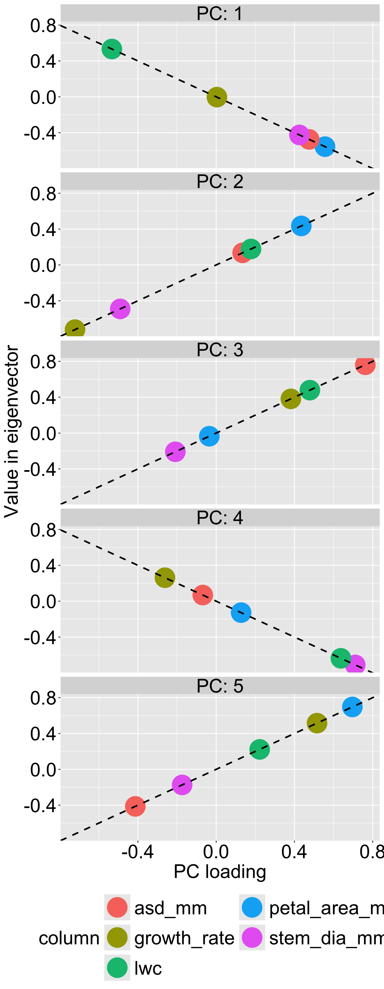
Figure 2: Comparing PCA loadings from prcomp() and eigenvectors from eigen(). Each panel shows one principal component (PC1–PC5). For each trait, the x-axis shows its loading from prcomp(), and the y-axis shows the corresponding value in the eigenvector from eigen(). The dashed lines indicate the near-perfect agreement between the two methods, differing only in sign. This demonstrates that (when everything is working right) prcomp() and eigen() produce equivalent results (up to sign) when the data are properly centered and scaled.
The trait loadings from eigenanalysis are basically the same as those from prcomp(). Figure 2 shows that, in our case, the trait loadings on each PC are the same, with the caveat that the sign may flips. This doesn’t change our interpretation (because PCs are relative, so sign does not matter), but is worth noting.
Find PC values by adding up each trait weighted by its loading
We already covered this.. If you like linear algebra, you can think about this as the dot product of the scaled and centered trait matrix and the matrix of trait loadings.
The problem(s) with missing data in PCA. Missing data causes two problems in PCA.
You cannot simply make a covariance or correlation matrix with missing data. This can be computationally overcome as follows cor( use = "pairwise.complete.obs"), but is only reliable if data are missing at random.
You cannot find PC values for individuals with missing data. Again there are computer tricks to overcome this, but they must be considered in the context of the data:
You can set missing values to zero. But this brings individuals with a bunch of missing values closer to the center of your PC plot.
You can drop individuals with missing data. But again, if patterns of missingness are non-random this can be a problem.
You can impute (smart guess) the missing values (using packages like missMDA, or mice) or use a PCA approach like emPCA or probabilistic PCA that do this for you. But then you are working on guesses of what your data may be and not what they are.
Why we usually scale our variables
We usually center and scale our variables so that our PC gives equal value to all variables. Sometimes we may not want to do this – perhaps we want to take traits with more variability more seriously. While this might be ok if variables are on very similar scales, it can be quite disastrous. Now that we’ve seen how PCA works using scaled data, let’s explore what happens when we skip the scaling step.
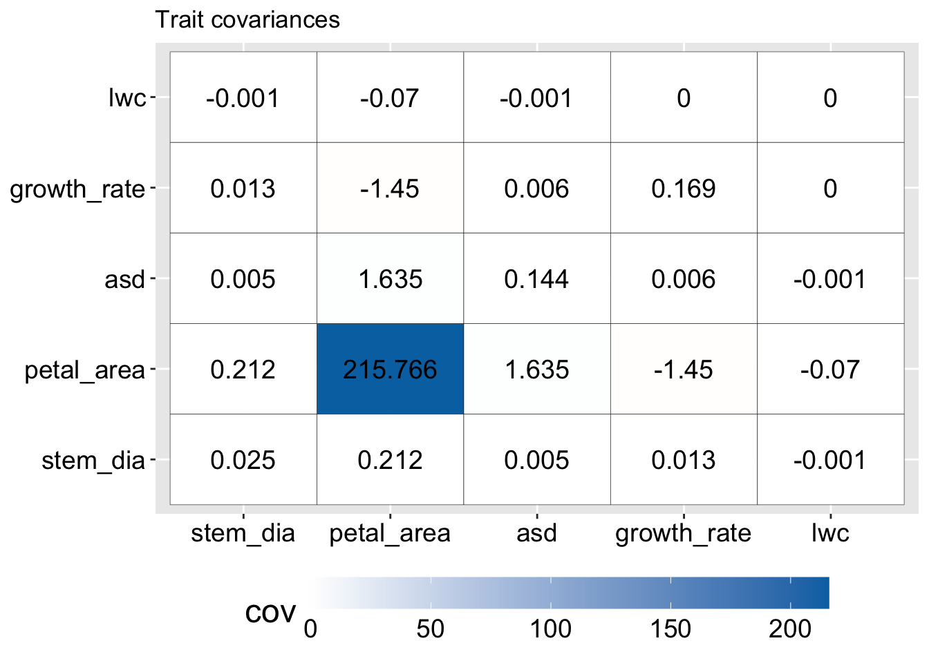
In our GC RIL data for example, petal area (measured in \(mm^2\)) has a much greater variance than any other trait (because the covariance of a variance with itself is the variance). You can see this on the main diagonal of Figure 3 where the variance in petal area is 216, while the second largest value in this matrix is less than two.
centered_gc_rils_4pca <- gc_rils_4pca |>select(-made_hybrid)|># Remove categorical variablesmutate_all(scale, scale =FALSE) # Subtract mean and divide by SD# Finding all pairwise covariances on centered (but not scaled) datacov_matrix <-cov(centered_gc_rils_4pca)
Figure 3: Covariance matrix of traits in parviflora RILS before scaling. Each cell shows the covariance between a pair of traits, with color indicating magnitude (darker blue = larger covariance). The diagonal shows trait variances. Petal area dominates the matrix with a variance over 215, while all other trait variances are below 2. This disparity illustrates how unscaled PCA can be overwhelmed by traits with larger absolute variation.
Now we can see the consequences of not scaling or centering on our PCs:
Becase the variance in petal area dominates the covariance matrix, PC1 explains 99.85% of the variability in the data (Table 1) and maps perfectly on to petal area (Table 2).
# Finding proportion # variance explained by PCgc_ril_centered_pca |>tidy(matrix ="pcs")