Motivating Scenario:
You have a fresh new dataset and want to check it out. Before providing numeric summaries you want to poke around the data so you are prepared to responsibly present appropriate summaries.
Learning Goals: By the end of this subchapter, you should be able to:
Identify the “skew” of data: You should be able to distinguish between:
Right skewed data – Most values small, some are very large.
Left skewed data – Most values large, some are very small.
Symmetric data – There are roughly as many small as large values.
Identify the number of modes in a data set. Differentiate between one, two and more modes.
Explain why we must consider the shape of data when summarizing it.
We start this chapter with bar plots and histograms instead of numerical summaries like the mean or variance because we must understand the shape of our data to properly present and interpret classic numeric summaries.
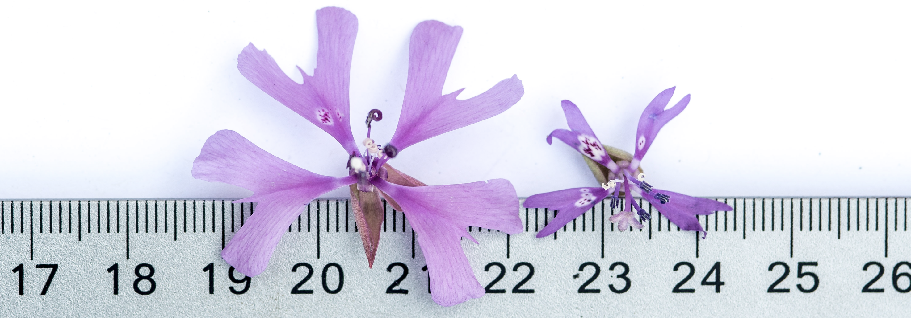
Figure 1: Measuring Clarkia xantiana flowers. Image from CalPhotos shared by Chris Winchell with a Creative Commons Attribution-NonCommercial-ShareAlike 3.0 (CC BY-NC-SA 3.0) license.
Skew
One key aspect of a dataset’s shape is skewness—whether the data is symmetrical or leans heavily toward smaller or larger values.
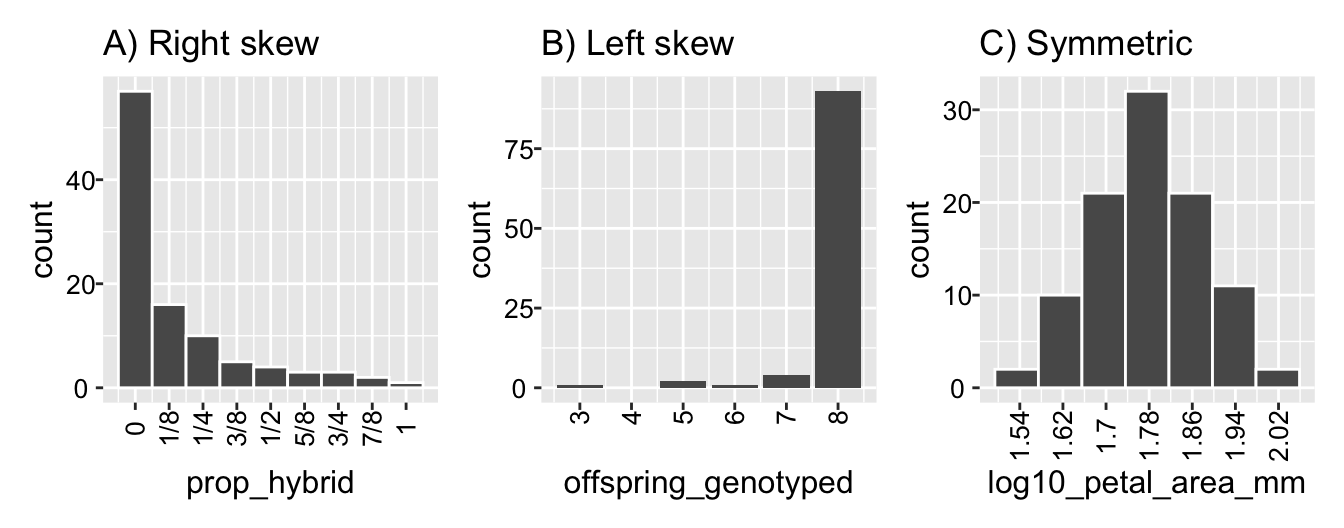
The proportion of hybrid seeds per RIL mom (Figure 4, and shown again in Figure 2 A) is strongly right-skewed—most values are small, but some are very large. Right-skewed data is common in biology and everyday life. For example, income is right-skewed: most people earn relatively little money, but some make loads of ca$h.
The number of offspring we genotyped (Figure 2 B) is strongly left-skewed—most values are large, but some are very small. Left-skewed data is also common in real-world settings. For example, age at death follows a left-skewed distribution: most people live long lives (often between 70 and 90), but some individuals die at much younger ages due to childhood mortality, diseases, accidents, or suicide.
The distributions in Figure 2 A and B represent extreme cases of skewness, where most values are either very small or very large. In contrast, Figure 2 C shows that on a \(\text{log}_{10}\) scale, petal area is nearly symmetric, with an even distribution of large and small values and most observations concentrated in the middle.
Figure 2: A bar plot showing the number of genotyped seeds of each mom shown to be hybrid.
Data transformations and skew:Figure 2 showed that \(\text{log}_{10}\) petal area was roughly symmetric. The careful might be suspicious and wonder why I transformed the data. The answer is that area is usually right skewed and log transforming often removes such skew.
We discuss changing the shape of distributions by transformation in the next section. Later we will see that symmetric data are often easier for statistical models than skewed data so such transformations are common.
Number of modes
One of the first things to notice when visualizing a dataset is whether the values cluster around a single peak or multiple peaks—this number of modes can reveal important patterns, such as distinct subgroups or natural variation in biological traits.
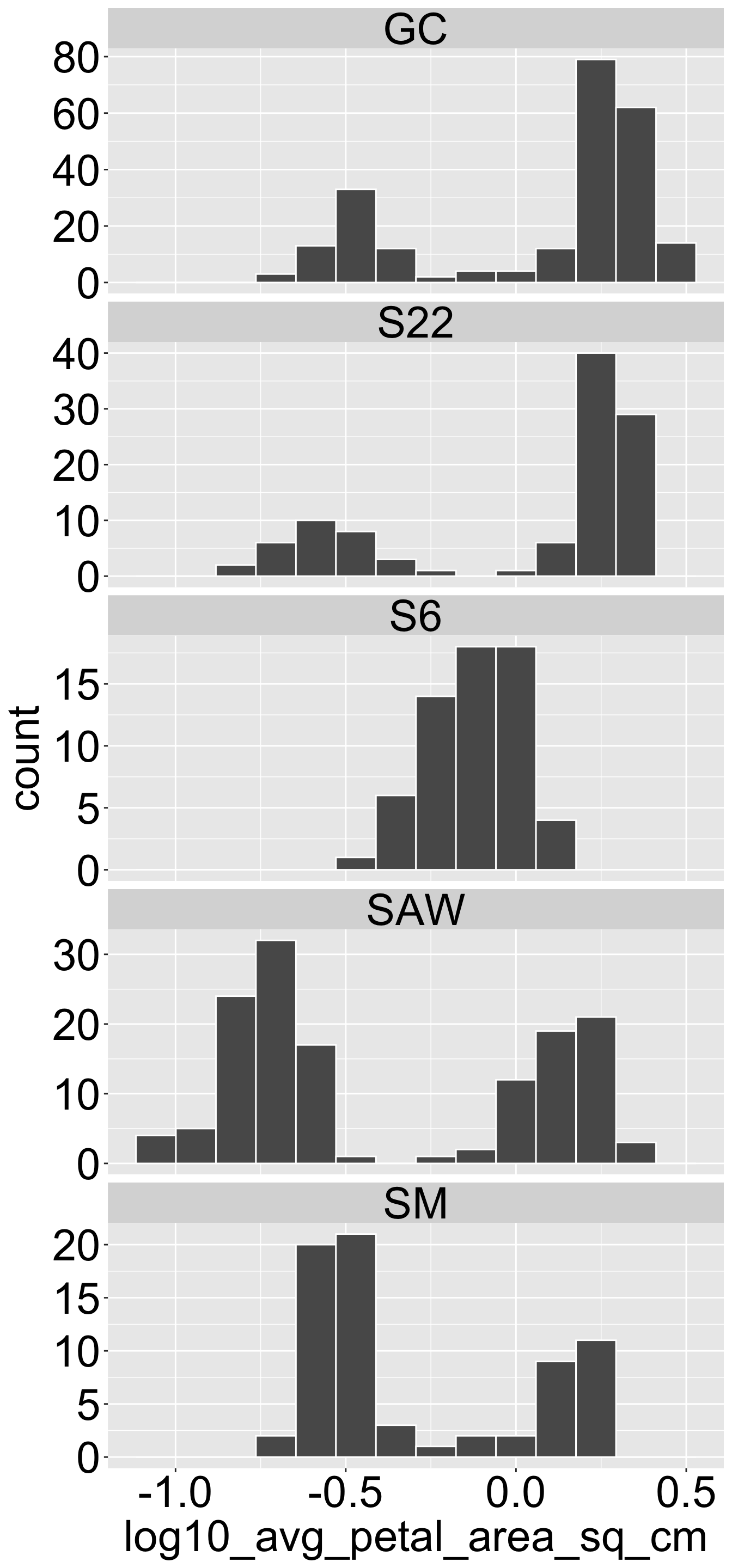
Figure 3: The distribution of petal area across four xantiana / parviflora hybrid zones. Data are available here.
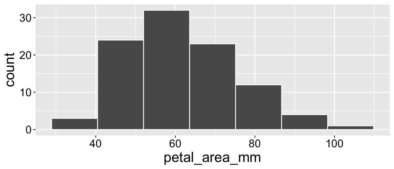
In unimodal distributions, there is a single, clear peak, with the number of observations in other bins decreasing as we move away from this central point. All distributions in Figure 2 are unimodal.
In bimodal distributions, there are two distinct peaks separated by a trough. Bimodal distributions are particularly interesting because they suggest that the dataset is composed of two distinct groups or categories.
Of course, distributions can have more than two modes. Trimodal distributions have three peaks, and so on. However, be careful not to over-interpret small fluctuations—small dips can create false peaks from random variation. It’s worth experimenting with bin sze to avoid overinterpreting such small blips.
The number of modes is particularly important in the study of speciation, especially in populations that may be hybridizing.
A unimodal hybrid zone suggests that two species merge when they come back into contact, implying they may not be distinct, stable species.
Bimodal or trimodal hybrid zones suggest that the two species largely maintain their distinctiveness when they have the opportunity to hybridize.
In a bimodal hybrid zone, the “trough” between peaks may include some hybrids.
In a trimodal hybrid zone, the middle peak might represent F1 hybrids.
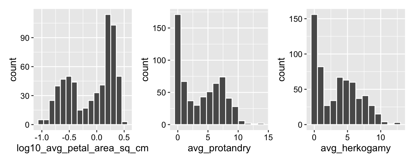
We were particularly interested in examining the distribution of phenotypes in seeds collected from parviflora / xantiana hybrid zones. Figure 4 shows that—unlike petal area in our RILs-most phenotypes from natural hybrid zones are largely bimodal. However, Figure 3 suggests that these distributions may themselves be a blend of different underlying distributions. While petal area appears bimodal in most populations, it may be unimodal at site S6. Figure 4 and Figure 3 highlight the benefit of digging into the data visually. We must visualize the distribution o values of a variable before we can provide a meaningful and interpretable summary statistic. .
Figure 4: Distributions of three floral traits in Clarkia xantiana hybrid zones: log10-transformed average petal area (sq. cm) (left), average protandry (middle), and average herkogamy (right). The petal area distribution is bimodal, with two distinct peaks. In contrast, both protandry and herkogamy are bimodal and strongly right-skewed, with most values clustered near zero and a secondary peak at higher values. These distributions suggest potential underlying biological structure, such as genetic variation or environmental influences shaping floral trait expression. Data are available here.