Motivating scenario: you want to limit your analysis to rows with certain values.
Learning goals: By the end of this sub-chapter you should be able to
Use the filter function to choose the rows you want to work with.
Display care so that you do not get the wrong answer when filtering your data.
Remove rows with filter()
There are reasons to remove rows by their values. For example, we could remove plants from US and LB locations. We can achieve this with the filter() function as follows:
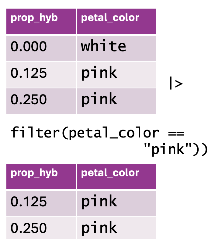
Figure 1: Using filter() to subset data based on a condition. The top table contains two columns: prop_hyb (proportion of hybrids) and petal_color (flower color), with values including both “white” and “pink” flowers. The function filter(petal_color == "pink") is applied to retain only rows where petal_color is “pink.” The resulting dataset, shown in the bottom table, excludes the “white” flower row and keeps only the observations where petal color is “pink.”
ril_data |> filter(location == "GC" | location == "SR"): To only retain samples from GC or (noted by |) SR. Recall that == asks the logical question, “Does the location equal SR?” So combined, the code reads “Retain only samples with location equal to SR or location equal to GC.”
OR, equivalently
ril_data |> filter(location != "US" & location != "LB"): To remove samples from US and (noted by &) LB. Recall that != asks the logical question, “Does the location not equal US?” Combined the code reads “Retain only samples with location not equal to US and with location not equal to LB.”
# rerunning the code summarizing visitation by # location and petal color and then ungrouping it# but filtering out plants from locations US and LB# note that the output no longer says `# Groups: location [2]`ril_data |>filter(location !="US"& location !="LB")|>group_by(location, petal_color) |>summarize(avg_vistis =mean(mean_visits, na.rm =TRUE),cor_visits_petal_area =cor(mean_visits ,petal_area_mm, use ="pairwise.complete.obs"))|>ungroup()
`summarise()` has grouped output by 'location'. You can override using the
`.groups` argument.
# A tibble: 6 × 4
  location petal_color avg_vistis cor_visits_petal_area
  <chr>    <chr>            <dbl>                 <dbl>
1 GC       pink            0.193                 0.0899
2 GC       white           0.0104                0.0886
3 GC       <NA>            0.2                   0.443
4 SR       pink            1.76                  0.387
5 SR       white           0.733                 0.458
6 SR       <NA>            1.04                  0.717
Warning… ! Remove one thing can change another:
Think hard about removing things (e.g. missing data), and if you do decide remove things, consider where in the pipeline you are doing so. Reoving one thing can change another. For example, compare: