• 7. linear model summary

A cartoon graph showing the number of T. rex limbs over time. 150 million years ago, T. rex had 4 limbs. By the time of extinction (~65 million years ago), it had "barely more than 2" limbs. A dashed line extrapolates this trend to today, humorously predicting a limbless, snake-like T. rex. Caption reads: "If T. rex hadn't gone extinct (Linear Extrapolation)." — Figure 1: If you keep extrapolating from data T. rex will into an absurd modern-day, snake-like dinosaur. This cartoon is adapted from xkcd. The original rollover text says: “Unfortunately, body size and bite force continue to increase”. See this link for a more detailed explanation.

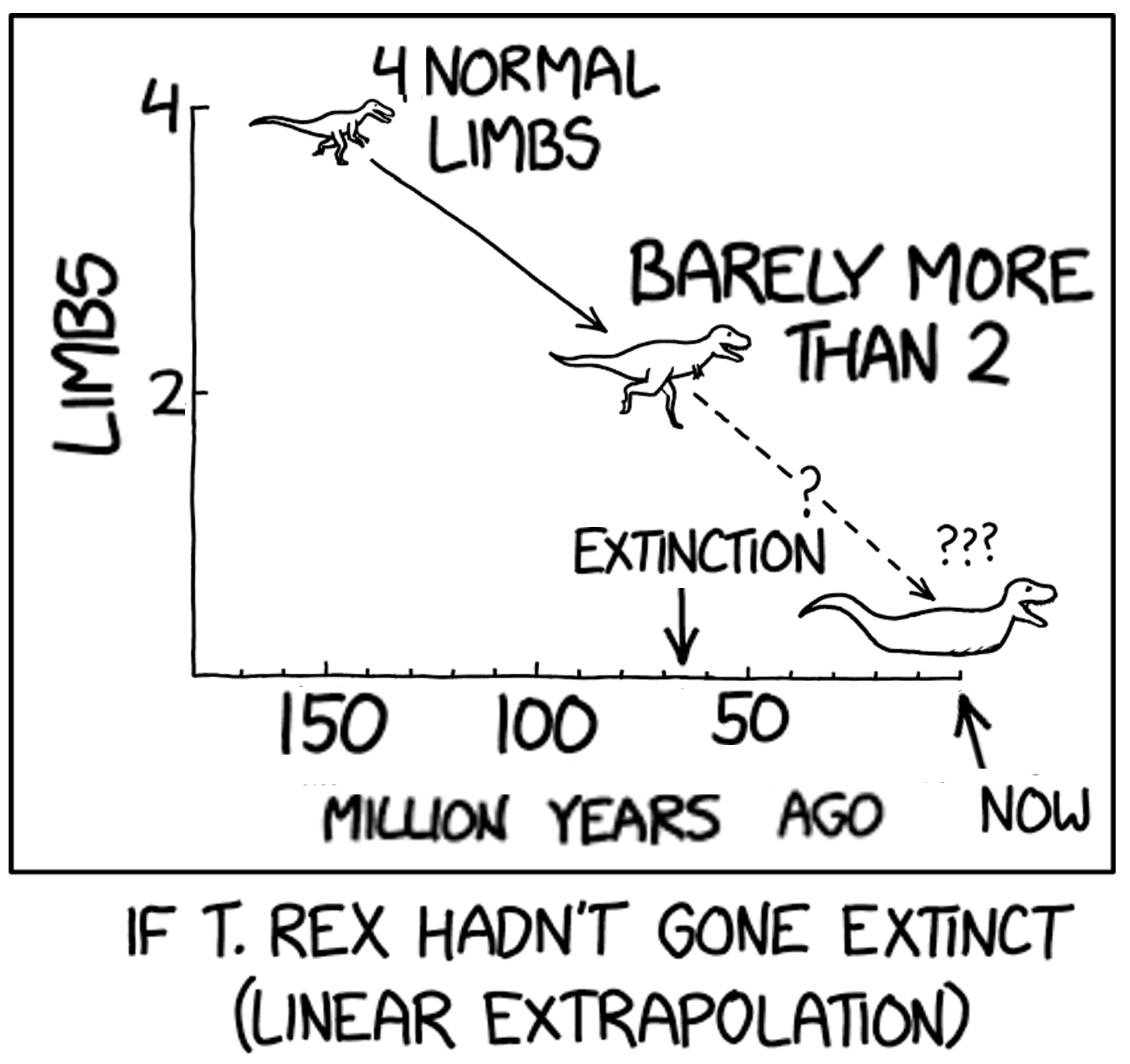
Links to: Summary. Questions. Glossary. R functions. R packages. More resources.

Linear models provide a unified framework for estimating the expected value (i.e., the conditional mean) of a numeric response variable as a function of one or more explanatory variables. These models are additive: the expected value is found by summing components of the model — the intercept plus the effect of each variable multiplied by its value. The sum of squared differences between observed values and predicted values describes how closely the data match the model’s predictions. Linear models can be descriptive tools that capture the structure, variation, and relationships in a dataset. In later chapters, we will build on this foundation to evaluate models more critically — assessing how well they fit, how reliable their predictions are, and how to diagnose their limitations.

Practice Questions

Try these questions! By using the R environment you can work without leaving this “book”. To help you jump right into thinking and analysis, I have loaded the ril data, cleaned it some, an have started some of the code!

Q1) What is the key difference between a scientific and a statistical model?

Statistical models make predictions, scientific models do not. Statistical models can be wrong, scientific models cannot. Statistical models describe patterns, scientific models are built on understanding processes. Statistical models make assumptions, scientific models do not. There are no differences between scientific and statistical models.

Q2 Consider the R code and output below. The (Intercept) describes:

The mean bill depth of penguins in this dataset. The mean bill depth of all penguins. The mean bill depth of penguins of the “reference level” species. The expected bill depth if all the predictors are set zero.

library(palmerpenguins)
lm(bill_depth_mm~1, penguins)


Call:
lm(formula = bill_depth_mm ~ 1, data = penguins)

Coefficients:
(Intercept)  
      17.15

Q3) Without running this code, predict which sex will be the reference level in the model: lm(bill_length_mm ~ sex, penguins)?

Q4 - Q7) Linear models with categorical predictors. The penguins data has data from three species of penguins – Adelie, Chinstrap and Gentoo. To answer the following questions, consider the R code and output below and no other information (that is, do not load these data into R).

lm(bill_length_mm~species, penguins)


Call:
lm(formula = bill_length_mm ~ species, data = penguins)

Coefficients:
     (Intercept)  speciesChinstrap     speciesGentoo  
          38.791            10.042             8.713

Q4) What is the mean bill length of Adelie penguins in the dataset?

Q5) What is the mean bill length of Chinstrap penguins in the dataset?

Q6) How many mm longer Chinstrap bills as compared to Gentoo bills in this dataset?

Q7) What is the mean bill length of all penguins in this dataset?

Q8 - Q13) Mathematics of linear regression. Use the summaries below to conduct a linear regression that models the response variable, bill depth, as a function of the explanatory variable, bill length.

mean_depth	mean_length	cov_length	sd_depth	sd_length
17.59	46.57	0.62	0.78	3.11

min_depth	max_depth	min_length	max_length	sample_size
16.4	19.4	40.9	58	34

Q8) The correlation between these variables is .

Q9) The slope in this model is .

Q10) The intercept in this model is .

Q11) According to the model, what is the predicted bill depth (in mm) for a penguin with a 50 mm long bill .

Q12) A penguin with a 20 mm deep and 50 mm long bill will have a residual of mm.

Q13) According to the model, what is the predicted bill depth for a penguin with a 500 mm long bill mm deep bill.

Of course you haven’t!! The correct answer, of course, is that you cannot predict outside the range of our data. See Figure 1!

Q14 - Q16) More than one explanatory variable. Use the summaries below to conduct a linear regression that models the response variable, bill depth, as a function of the explanatory variable, bill length.

library(ggplot2)
library(dplyr)
library(palmerpenguins)
library(broom)


gentoo_data <- penguins        |>
  filter(species == "Gentoo") 

lm(bill_depth_mm ~ bill_length_mm +sex, data = gentoo_data)|>
  augment() |>
  ggplot(aes(x=bill_length_mm , y=bill_depth_mm,color = sex))+
  geom_point(size = 5, alpha = .7)+
  geom_smooth(method = "lm",se = FALSE, linetype = "dashed",linewidth = 2)+
  geom_smooth(aes(y = .fitted), se=FALSE, linewidth = 2)+
  theme(legend.position = "top", 
        axis.title  = element_text(size = 28),
        axis.text   = element_text(size = 28),
        legend.text = element_text(size = 28),
        legend.title = element_text(size = 28))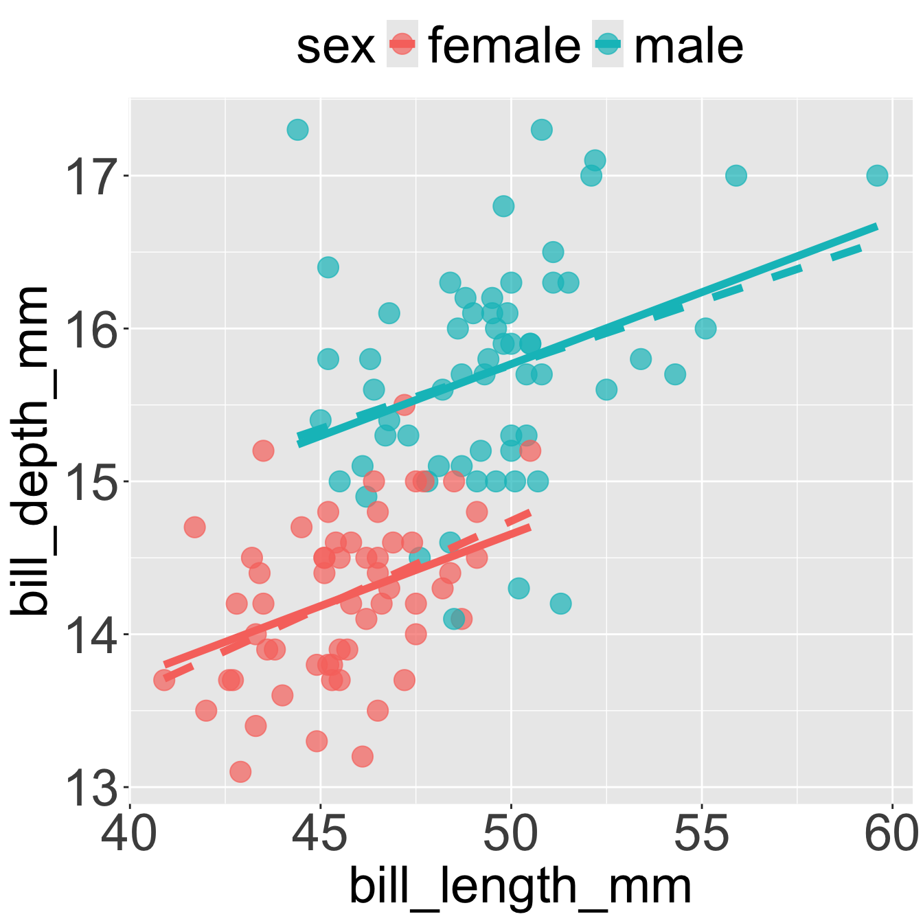

Scatterplot of Gentoo penguin bill length (x-axis) versus bill depth (y-axis), colored by sex (red = female, blue = male). Each point represents an individual. Solid lines show model-predicted bill depth based on bill length and sex. Dashed lines show simple linear regression fits for each sex. Male Gentoo penguins generally have deeper bills than females, and bill depth increases slightly with bill length for both sexes. — Figure 2: **Bill depth as a function of bill length for Gentoo penguins, separated by sex.** Solid lines show the predicted values from a multiple regression model including both bill length and sex as predictors. Dashed lines show simple linear fits ignoring other predictors. The plot highlights both the overall trend with bill length and differences in mean depth between males and females.

Q14) In Figure 2 there is a male penguin with a bill that is about 56 mm long (the second most extreme right point). Approximate, by eye its residual.

Q15) Based on Figure 2, which of the following are nearly identical for male and female Gentoo penguins? (Select all that apply.)

Mean bill lengths Mean bill depths Slopes Intercepts This plot shows that nearly nothing is nearly identical between male and female Gentoo penguins

Q16) Use the web R space above to model flipper length as a function of body mass and sex of Chinstrap penguins. The sum of squared residuals is:.

📊 Glossary of Terms

📚 1. Concepts of Modeling

Statistical Model: A mathematical description of patterns in data, often used to summarize, predict, or test hypotheses.
Scientific Model: A conceptual model based on biological understanding, explaining processes in the real world.

🔀 2. Different Predictor Types

Categorical Predictor: A variable with discrete groups. Modeled by differences in intercepts across groups.
Numeric Predictor: A continuous variable. Modeled by slopes showing expected change in the response per unit change in the predictor.
Indicator Variable: A numeric coding of a categorical variable (e.g., 0 for “pink,” 1 for “white”).
Reference Level: The baseline category in a categorical predictor against which other groups are compared.

3. Components of a Linear Model

Conditional Mean, \(\hat{y}_i\): The predicted value of a response variable for given explanatory variable values.
- General linear model form: \(\hat{Y}_i = f(\text{explanatory variables}_i)\).
- Linear combination form: \(\hat{Y}_i = b_0 + b_1 x_{1,i} + b_2 x_{2,i} + \dots + b_k x_{k,i}\).
Intercept (b₀): The expected value of the response when all explanatory variables are zero (sometimes called \(a\)).
Slope (b₁): The expected change \(\hat{y}_i\) with change in the predictor.
- For numeric predictor: The expected change in the response for a one-unit increase in a numeric explanatory variable. \(b_1 = \text{cov}_{x,y}/\sigma^2_x\).
- For binary predictor: The difference in the meane of non reference and reference level.
\(x_{1,i}\) The value of explantory variable, \(1\), in individual \(i\).
- For numeric predictors: The value of the explanatory variable.
- For binary predictors: The value of the indicator variable.
  - \(x_1\) equals 0 for the reference group.
  - \(x_1\) equals 1 for the non-reference group.

4. Concepts for Linear Models.

Observed value (yᵢ): The actual value of the response variable: \(y_i = \hat{y}_i +e_i\).
Residual (eᵢ): The difference between an observed value and its model-predicted value, \(e_i = y_i-\hat{y}_i\).
Residual Sum of Squares: \(\sum e_i^2\)
Residual Standard Deviation: A measure of typical residual size — how far off predictions tend to be \(\sum e_i^2/(n-1)\).

🚫 5. Model Limitations

Extrapolation: Making predictions outside the range of observed data — generally unsafe.
Multicollinearity: When explanatory variables are highly correlated, making it hard to separate their individual effects.

Key R Functions

📈 Building Linear Models

lm(): Fits linear models. Syntax: lm(response ~ explanatory, data = dataset).
augment() ([broom]): Adds predictions and residuals to your dataset for easy exploration.

R Packages Introduced

broom: Tidies model outputs (like fitted values and residuals) into neat data frames.
ggplot2: Used for visualizing data and model fits.