ril_data      |>
  summarize(avg_visits = mean(mean_visits))
# A tibble: 1 × 1
avg_visits
<dbl>
1 NAMotivating scenario: you want to get summaries of your data.
Learning goals: By the end of this sub-chapter you should be able to
summarize()ing dataWe rarely want to look at entire datasets, we want tosummarize() them (e.g. finding the mean, variance, etc..).
We previously used the mean function to find the mean of a vector. When we want to summarize a variable in a tibble we use the function inside of summarize()
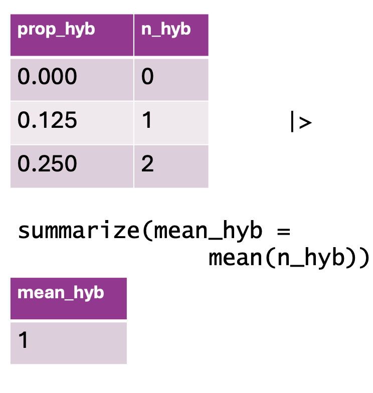
summarize(). The top table contains two columns: prop_hyb (proportion of hybrids) and n_hyb (the number of hybrids). The summarize(mean_hyb = mean(n_hyb)) function is applied to calculate the mean of n_hyb, producing a single-row output where mean_hyb represents the average number of hybrids across the dataset. The final result, shown in the bottom table, contains a single value of 1.ril_data |>
summarize(avg_visits = mean(mean_visits))# A tibble: 1 × 1
avg_visits
<dbl>
1 NAWe notice two things.
The answer was NA. This is because there are NAs in the data.
The results are a tibble. This is sometimes what we want and sometimes not. If you want a tibble you can pull() the value.
Summarize data in the face of NAs with the na.rm = TRUE argument.
ril_data      |>
  summarize(avg_visits = mean(mean_visits, na.rm = TRUE))
# A tibble: 1 × 1
avg_visits
<dbl>
1 0.693pull() columns from tibbles to extract vectors.
Many R functions require vectors rather than tibbles. You can pull() them out as follows:
ril_data      |>
  summarize(avg_visits = mean(mean_visits, na.rm = TRUE))|>
  pull()
[1] 0.693259
group_by() andsummarize() to describe groupsSay we were curious about differences in pollinator visitation by location. The code below combines group_by() and summarize() to show that site SR had nearly 10 times the mean pollinator visitation per 15 minute observation than did site GC. We also see a much stronger correlation between petal area and visitation in SR than in GC, but a stronger correlation between proportion hybrid and visitation in GC than in SR. Note that the NA values for LB and US arise because we did not conduct pollinator observations at those locations.
ril_data      |>
  group_by(location) |>
  summarize(grand_mean = mean(mean_visits, na.rm = TRUE),
            cor_visits_petal_area =  cor(mean_visits ,petal_area_mm,
                use = "pairwise.complete.obs"),
            cor_visits_prop_hybrid =  cor(mean_visits , prop_hybrid,
                use = "pairwise.complete.obs")) # Like na.rm = TRUE, but for correlations
# A tibble: 5 × 4
location grand_mean cor_visits_petal_area cor_visits_prop_hybrid
<chr> <dbl> <dbl> <dbl>
1 GC 0.116 0.0575 0.458
2 LB NaN NA NA
3 SR 1.27 0.367 0.281
4 US NaN NA NA
5 <NA> NaN NA NA We can group by more than one variable. Grouping by location and color reveals not ony that white flowers are visited less than pink flower, but also that petal area has a similar correlation with pollinator visitation for pink and white flowers.
ril_data      |>
  group_by(location, petal_color) |>
  summarize(avg_visits = mean(mean_visits, na.rm = TRUE),
            cor_visits_petal_area =  cor(mean_visits ,petal_area_mm,
                use = "pairwise.complete.obs")) # Like na.rm = TRUE, but for correlations
`summarise()` has grouped output by 'location'. You can override using the
`.groups` argument.# A tibble: 13 × 4
# Groups: location [5]
location petal_color avg_visits cor_visits_petal_area
<chr> <chr> <dbl> <dbl>
1 GC pink 0.193 0.0899
2 GC white 0.0104 0.0886
3 GC <NA> 0.2 0.443
4 LB pink NaN NA
5 LB white NaN NA
6 LB <NA> NaN NA
7 SR pink 1.76 0.387
8 SR white 0.733 0.458
9 SR <NA> 1.04 0.717
10 US pink NaN NA
11 US white NaN NA
12 US <NA> NaN NA
13 <NA> <NA> NaN NA 
After summarizing, the data above are still grouped by location. You can see this under #A tibble: 6 x 4 where it says # Groups: location [5]. This tells us that the data are still grouped by location (these groups correspond to GC, SR, US, LB and missing location information NA). It’s good practice to ungroup() next, so that R does not do anything unexpected.
Peeling of groups: Above we grouped by location and petal_color in that order. When summarize data, by default, R peels off one group, following a “last one in is the first one out” rule. This is what is meant when R says: “summarise() has grouped output by ‘location’…”.
# re-running code above and then ungrouping it.
# note that the output no longer says `# Groups:   location [2]`
ril_data      |>
  group_by(location, petal_color) |>
  summarize(avg_vistis = mean(mean_visits, na.rm = TRUE),
            cor_visits_petal_area =  cor(mean_visits ,petal_area_mm,
                use = "pairwise.complete.obs"))|>
  ungroup()
`summarise()` has grouped output by 'location'. You can override using the
`.groups` argument.# A tibble: 13 × 4
location petal_color avg_vistis cor_visits_petal_area
<chr> <chr> <dbl> <dbl>
1 GC pink 0.193 0.0899
2 GC white 0.0104 0.0886
3 GC <NA> 0.2 0.443
4 LB pink NaN NA
5 LB white NaN NA
6 LB <NA> NaN NA
7 SR pink 1.76 0.387
8 SR white 0.733 0.458
9 SR <NA> 1.04 0.717
10 US pink NaN NA
11 US white NaN NA
12 US <NA> NaN NA
13 <NA> <NA> NaN NA