7 Linear Models as Summaries
Motivating Scenario: You want to move beyond simply plotting and summarizing associations and start modeling relationships between variables.
Learning Goals: By the end of this chapter, you should be able to:
Explain what a linear model is and what it does.
- Understand a linear model as a way of estimating the conditional mean of a response variable.
Interpret the components of a linear model
Explain the meaning of intercepts, slopes (effect sizes), and predicted values.
Define and interpret residuals and the residual standard deviation.
Estimate a slope from a dataset with math and with R.
Estimate a conditional mean from a linear model with multiple explanatory variables.
In this section, we’ll introduce statistical models as simplified descriptions of the world. You’ll notice that you’re already familiar with some simple models. For example, the mean and variance provide a basic model for a single continuous variable, while a conditional mean and pooled variance describe a continuous response variable with a categorical explanatory variable.
7.1 Statistical models are not scientific models
This is a BIOstatistics book. It is written by and for biologists interested in biological ideas. We are inspired by biological questions generated by scientific understanding and scientific models of the world. However, a major way in which we evaluate such scientific models is via statistical models and hypotheses. Confusing a statistical model for a scientific model is a common and understandable mistake that we should avoid. Scientific models and statistical models are different:
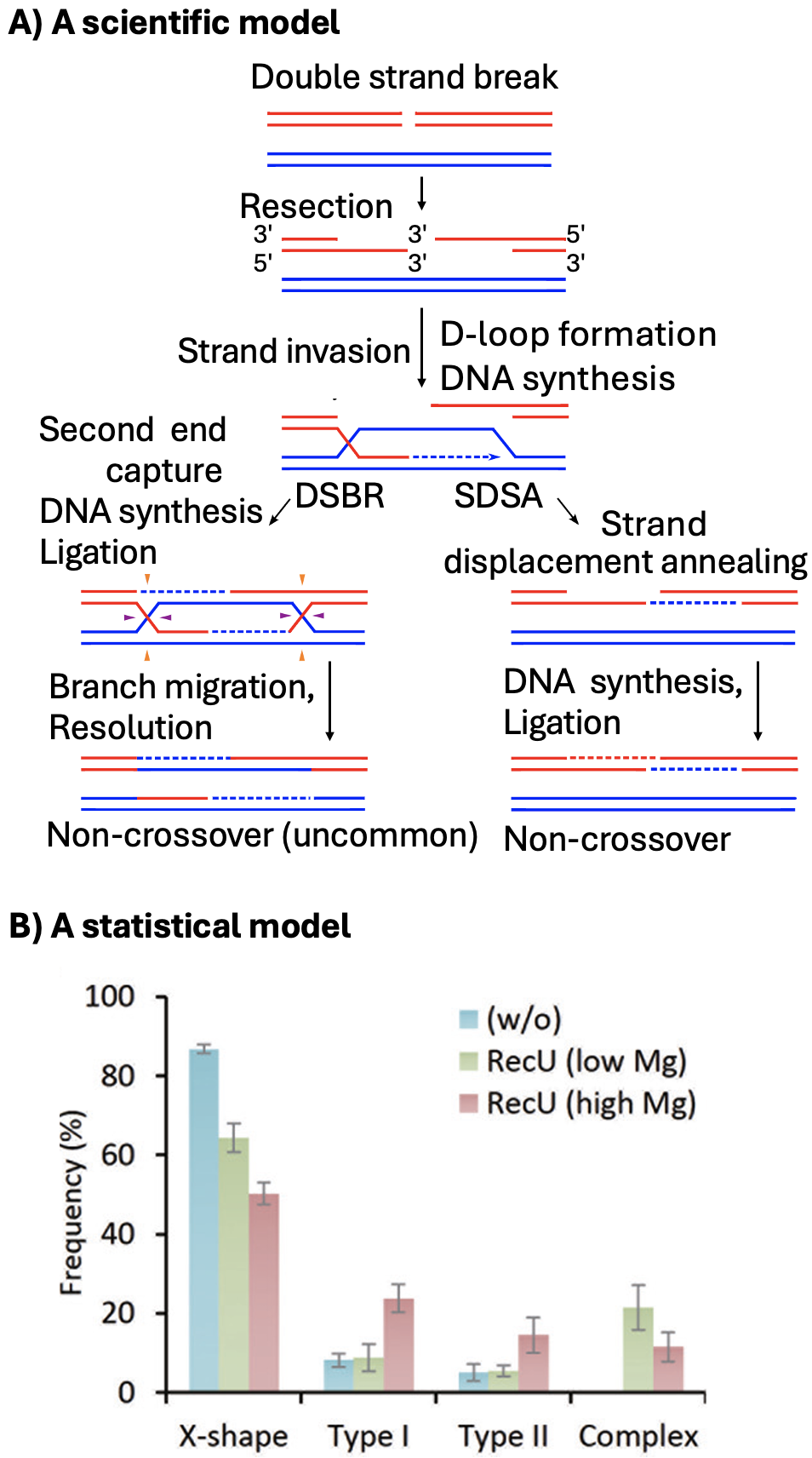
Scientific models are based on our understanding of the science – in this case biology. Biological models come from us making simplified abstractions complex systems (like considering predator-prey interactions, plant pollination, cancer progression, or meiosis (Figure 7.1 A)). Great scientific models explain what we see, make interesting predictions, and are consistent with our broader scientific understanding.
Statistical models on the other hand, are mathematical ways to describe patterns in data (e.g. Figure 7.1 B). Statistical models know nothing about Lotka-Voletera, pollination or human physiology.
Because statistical models know nothing about science it is our job to build scientific studies best suited for clean statistical interpretation, build statistical models that best represent our biological questions, and interpret statistical results as statistical. We must always recenter biology in interpreting any statistical outcome.
7.1.1 Scientific & statistical models: The Clarkia case study
In our Clarkia example, the big-picture scientific model is that when parviflora came back into contact with its close relative, xantiana, it evolved traits — such as smaller petals — to avoid hybridizing with xantiana. No single statistical model or study fully captures this scientific model. Instead, we design experiments to evaluate pieces of the model. For example, we:
Compare petal area between parviflora plants from populations that occur with xantiana (sympatric populations) and those from populations far away from xantiana (allopatric populations).
Conduct an experiment by planting individuals from sympatric and allopatric parviflora populations in the same environment as xantiana, and comparing the amount of hybrid seed set by plants from each origin.
Generate Recombinant Inbred Lines (RILs) between sympatric and allopatric parviflora populations, and examine whether petal area is associated with the proportion of hybrid seeds produced.
As you can see, statistical models don’t “know” anything about biology — they simply describe patterns in data. It’s up to us, as biologists, to design experiments carefully, choose the right statistical models, and interpret results in light of our biological hypotheses.
7.2 Linear models
Linear models are among the most common types of statistical model. Linear models estimate the conditional mean of the \(i^{th}\) observation of a continuous response variable, \(\hat{Y}_i\) for a (combination) of value(s) of the explanatory variables (\(\text{explanatory variables}_i\)):
\[\begin{equation} \hat{Y}_i = f(\text{explanatory variables}_i) \end{equation}\]
Conditional mean: The expected value of a response variable given specific values of the explanatory variables (i.e., the model’s best guess for the response based on the explanatory variables).
These models are “linear” because we get this estimate of the conditional mean, \(\hat{Y}_i\), by adding up all components of the model. That is, each explanatory variable \(y_{j,i}\) is multiplied by its effect size \(b_j\). So, for example, \(\hat{Y}_i\) equals the parameter estimate for the “intercept”, \(a\) plus its value for the first explanatory variable, \(y_{1,i}\), times the effect of this variable, \(b_1\), plus its value for the second explanatory variable, \(y_{2,i}\) times the effect of this variable, \(b_2\), and so on for all included predictors.
\[\begin{equation} \hat{Y}_i = a + b_1 y_{1,i} + b_2 y_{2,i} + \dots{} \end{equation}\]
OPTIONAL / ADVANCED, FOR MATH NERDS:. If you have a background in linear algebra, it might help to see a linear model in matrix notation.
The first matrix below is known as the design matrix. Each row corresponds to an individual, and each entry in the \(i\)th row corresponds to that individual’s value for a given explanatory variable. We take the dot product of this matrix and our estimated parameters to get the predictions for each individual. The equation below has \(n\) individuals and \(k\) explanatory variables. Note that every individual has a value of 1 for the intercept.
\[\begin{equation} \begin{pmatrix} 1 & y_{1,1} & y_{2,1} & \dots & y_{k,1} \\ 1 & y_{1,2} & y_{2,2} & \dots & y_{k,2} \\ \vdots & \vdots & \vdots & \ddots & \vdots \\ 1 & y_{1,n} & y_{2,n} & \dots & y_{k,n} \end{pmatrix} \cdot \begin{pmatrix} a \\ b_{1}\\ b_{2}\\ \vdots \\ b_{k} \end{pmatrix} = \begin{pmatrix} \hat{Y}_1 \\ \hat{Y}_2\\ \vdots \\ \hat{Y}_n \end{pmatrix} \end{equation}\]
7.3 Residuals and Variance in Linear Models
As with a simple mean, actual observations usually differ from their predicted (conditional mean) values.
The difference between an observed value for an individual (\(Y_i\)) and the predicted value from the linear model (\(\hat{Y}_i\)) is called the residual, \(e_i\):
Residual: The difference between an observed value and its predicted value from a linear model (i.e., the conditional mean given that observation’s values for the explanatory variables).
\[e_i = Y_i - \hat{Y}_i\]
You can also rearrange this to think about it the other way around:
\[Y_i = \hat{Y}_i + e_i\]
Just like when we summarized variability around a simple mean, we can summarize variability around a model’s predictions by looking at the spread of the residuals. That is, linear models don’t just give us a conditional mean — they also give us a way to estimate how much observations tend to vary around that mean.
We calculate the residual variance (and residual standard deviation) of the residuals like this:
\[\text{Residual variance} = \frac{ \sum e_i^2}{n-1}\]
A small caveat: This equation is a bit off — the denominator should actually be \(n - p\), where \(p\) is the number of parameters estimated in our model (including the intercept). But it’s close enough for now. We can worry about being precise later — in much of statistics, being approximately right is good enough.
\[\text{Residual standard deviation} = \sqrt{\frac{\sum e_i^2}{n-1}}\] :::aside Residual standard deviation: The typical size of a residual — that is, how far observed values tend to fall from their predicted values in a linear model. :::
Again, we can think of the residual standard deviation as telling us, on average, how far away from their predicted value individuals are expected to be. In fact, when we calculated the pooled standard deviation earlier, we were already doing a special case of what we now call the residual standard deviation — just in the simple situation of two groups.
7.4 Assumptions, Caveats and our limited ambitions
In this section, we focus on building and interpreting linear models as descriptions of data. We will put off a formal discussion of what makes a linear model reasonable — and how to diagnose whether a model fits its assumptions — until later. In the meantime, as we build and interpret models, we’ll keep an informal eye out for clues that something might be wrong — but we’ll learn formal tools to evaluate if if a specific model meets assumptions of a linear model later.
This doesn’t mean that interpreting linear models is more important than evaluating whether they are any good (in fact, in real research, interpreting and evaluating models are inseparable). It just means it’s hard to teach a bunch of interconnected ideas and approaches all at once — and after years of experimentation, I’ve found this approach to be the most successful. That said, before you conduct any serious linear modeling work, you should definitely jump ahead and read PART XXX of this book, where we discuss model assumptions and how to check them carefully.
Integrate Clarkia as a model – reinforcement.
Bit about hypotheses
- conditional means
- we have seen this lets for it oncece for hyb as function of petal color
- revisit pooled variance
More than one level - now numerous. levels (say sight?)
- continuous predictor
- a slope
- minimizing SS of Squares
- SS_ model and r^2
- one continuous, one categorical predictor
- and more!