Motivating Scenario: You have a dataset with many variables (e.g. Numerous prototypes, RNA Seq, large scale genomic or phenomic data, OTU coutns etc…) and want to broadly summarize variability in this dataset and the associations between these many variables. However, there are too many variables to interpret with simple plots or pairwise comparisons. You need a way to summarize the patterns of variation across all traits simultaneously.
Learning Goals: By the end of this chapter, you should be able to:
Understand what ordination methods like PCA and NMDS do
Explain the goals of PCA and NMDS in summarizing multivariate patterns.
Interpret PCA results in biological terms
Describe how traits combine to form principal components
Quantify how much variance is explained by each component
Understand and compare PCA and NMDS
Know when PCA is appropriate and when NMDS might be better
Anticipate and avoid common pitfalls
Handle missing data, decide whether to scale variables, and recognize when you’re double-counting information
Modern biology generates rich, high-dimensional data. A single study we might measure dozens of traits, behaviors, or molecular features per individual. Grinding up samples and running them through various macines provides us with genotypes at millions of loci, measures of gene expression across tissues, characterization of the thousands of microbes in a sample etc. Trying to interpret each variable on its own quickly becomes overwhelming — and looking at pairs of traits one at a time misses the bigger picture. To truly understand variation in multivariate data, we need tools that summarize how individuals differ across all traits simultaneously.
Here’s a lightly edited version for clarity and flow:
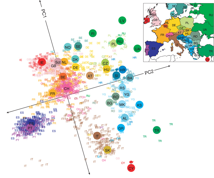
A common set of tools, known as ordination methods, summarize high-dimensional datasets into a few major axes of variation. These summaries can be incredibly informative, revealing key patterns in the data. For example, John Novembre showed that summarizing whole-genome data by its major axes of variation revealed a structure in European genetic variation that closely mirrors the geographic map of Europe.
by finding combinations of the original variables that capture the dominant patterns in the data. They help us zoom out and see broad trends: which individuals are similar, which traits vary together, and whether groups of individuals separate in trait space.
library(ggfortify)
In this chapter, we’ll begin with Principal Component Analysis (PCA) — a linear method that looks for the directions of greatest variance in your data. We’ll use a familiar dataset: Clarkia individuals from the GC site, for which we’ve measured anther-stigma distance, petal area, and leaf water content. These traits may relate to different aspects of plant performance or pollination biology — but PCA won’t “know” that. It will simply tell us how plants vary.
Later, we’ll explore Non-metric Multidimensional Scaling (NMDS), which takes a different approach. NMDS focuses on preserving pairwise similarities, even when the relationships among traits are complex and nonlinear. Where PCA excels at finding big trends, NMDS is often better at capturing subtle relationships based on ecological distance.
But before we jump into methods, we’ll make sure we understand what these tools are summarizing. We’ll start with PCA — how it works, what it tells us, and how to interpret it thoughtfully. Along the way, we’ll also wrestle with practical questions: - What do we do about missing data? - Should we scale our variables? - When are two variables redundant?
Ordination is a tool. It helps us simplify — but it also demands thoughtful decisions and interpretation.